Revenue Sensitivity
The Problem
In mobile advertising, it's well understood that performance experiences diminishing returns as customer spend increases. Our machine learning models prioritize the highest-quality user segments, those most likely to convert, and progressively move into lower-performing segments as budget scales. This creates a natural trade-off: while we aim to unlock higher budgets, our customers will quickly pull back if performance declines below target.
Often times, we find that we're exceeding performance goals but unable to secure additional budget due to concerns about performance degradation. In these cases, having a way to forecast a spend level that aligns with the customer's goals is invaluable. To address this, we needed a structured way to model the relationship between customer spend and the performance return for any given campaign. A model like this would enable us to identify the inflection point of our customer’s goal, and equip our commercial team with data-driven answers to our customers’ questions.
How I Solved It
To better understand the relationship between customer spend and performance, I developed a custom Explore in Looker that visualizes a logarithmic regression line between weekly spend and downstream performance metrics. The underlying dataset spans a full year of campaign data and is grouped by week to align with how our customers allocate budgets. The regression itself is computed within a derived table, with Looker parameters driving the logic inside the innermost CTE. These parameters allow users to dynamically toggle between cohorted and uncohorted data sources, and to simulate adjustments to revenue or margin assumptions directly within the dashboards.
While the resulting dashboards are powerful and flexible, their usefulness is dependent on a nuanced understanding of the data. Because misinterpretation could lead users to make confident but incorrect decisions, I implemented guardrails. Access to the Explore is limited to a vetted group of Looker power-users who received walkthroughs and context on its intended use. The dashboards themselves were moved to permission-managed folders to maintain control over visibility and ensure that decision-making remains informed and responsible.
The Core Resulting Dashboard
One of the key deliverables from this Explore was the Margin Sensitivity Dashboard, which enables users to simulate performance outcomes based on hypothetical Gross Revenue and margin inputs. In performance marketing, the net revenue margin is the proportion of Gross Revenue withheld. The remaining portion of revenue reinvested on the customer’s behalf to drive user acquisition and down-funnel performance is known as spend. Modeling on spend is critical, as it reflects the true scale of investment and its impact on performance.
By incorporating margin directly into the modeling logic, the dashboard accounts for scenarios where increased Gross Revenue could be offset by a higher margin, resulting in flat or even reduced spend. This nuance is essential, as spend, not Gross Revenue, is the primary driver in our regression model. Users can explore how changes to margin affect key metrics like Installs, Events, or Customer Revenue, making this a powerful tool for tradeoff analysis. It also supports strategic decision-making, whether the goal is to maximize Net Revenue, improve campaign performance, or finding equilibrium between rising budgets and degrading performance.
The user’s inputs are converted into a projected spend value, which is then fed into the regression model to estimate downstream KPIs. Each simulation is visualized alongside historical data points, with predicted values plotted on the same scale. R² values are embedded as error bars, encouraging users to assess the model’s fit visually before drawing conclusions. This design ensures transparency while empowering commercial and operations teams to engage in more data-informed planning and scenario modeling.
Flexibility through parameters

Dashboard users update parameters and filters to narrow in on a campaign, and compare different Revenue-Margin tuples. Within the same view, users can view the observed data from the most recent week, the model’s prediction of performance for the current combination of revenue and margin, and calculated metrics from a proposed change.

The user inputted values resolve to create the estimated KPIs, classifications, and comparisons above
Confidence is a classification of the R-squared value, where values lower than 0.70 are classified as “Low”
Sensitivity measures how sensitive a campaign would be to a revenue/margin change, the more sensitive a campaign is, the more volatile changes to performance will be as a result of changes
The ‘historical’ values are predicted metrics based on historic data. The name historic was chosen to reinforce that this tool is based on historic data, and will not account for recent changes made to the campaign.
The ‘incremental’ RPI in this instance, is the cost of driving each incremental install at the spend level chosen. It is calculated by taking the derivative of the regression at the user’s spend level for an instantaneous rate of change. This is a brand new idea for my team, which typically views the average cost per install (CPI).
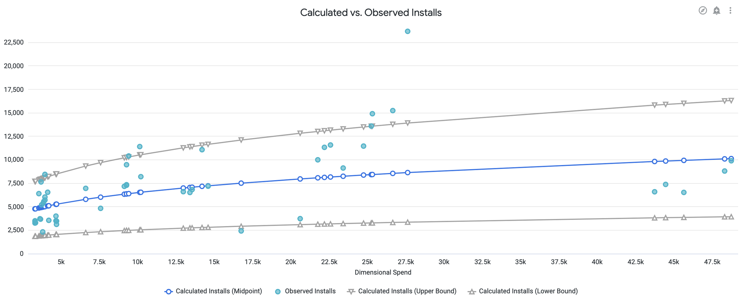
The dashboard also provides a visual representation of the model’s fit. A user who is interested in this campaigns performance at the $25k spend/week level, might expect this model to under-predict performance, while a user at the $45k/week spend level might expect the model to over-predict performance.
The Innermost CTE:
The innermost CTE in this workflow is intentionally lightweight and flexible, using LookML parameters to dynamically modify the underlying SQL. These parameters control both the campaign_id filter, enabling users to isolate a single campaign, and a toggle to switch between cohorted and uncohorted (spot) data sources by changing the referenced source table. Conditional logic is employed to ensure that only valid fields are selected based on the chosen source, avoiding errors from referencing non-existent columns.
This flexibility is critical because different customers evaluate performance in different ways: some prioritize cohorted metrics for their consistency, while others prefer uncohorted metrics to see the full extent of performance driven. By allowing the user to adjust whether the source data is cohorted or not, we are able to align the model with how our customers evaluate our performance.
Importantly, LookML parameters enable us to change the actual query structure, rather than simply applying filters post-aggregation. Without this capability, we would be forced to include all live campaign data in both a cohorted and uncohorted view—massively increasing the resource requirements. Instead, this approach keeps the logic consolidated and efficient. Because querying a year’s worth of campaign data at the weekly grain is relatively lightweight, this method reduces processing overhead while improving the responsiveness the Explore.
WITH lobf_prep AS (
  SELECT
      campaign_id
  {% if table._parameter_value == 'schema.table_name' %}
      , SUM(rev_micros) / 1000000 AS revenue
      , SUM(spend_micros) / 1000000 AS spend
      , SUM(conv_events) AS events
      , SUM(installs_count) AS installs
  {% else %}
      , SUM(rev_micros_d7) / 1000000 AS revenue
      , SUM(spend_micros) / 1000000 AS spend
      , SUM(conv_events_d7) AS events
      , SUM(installs_count_d7) AS installs
  {% endif %}
  {% if table._parameter_value == 'schema.table_name_attr' %}
      , SUM(cust_rev_micros_d7) / 1000000 AS cr
  {% else %}
      , NULL AS cr
  {% endif %}
      , CAST(date_trunc('week', from_iso8601_timestamp(log_date)) AS DATE) AS week
  FROM
    {{ table._parameter_value }}
  WHERE 1 = 1
    AND exclude_flg <> 'true'
    AND campaign_id = {{ campaign_id._parameter_value }}
    AND from_iso8601_timestamp(log_date) >= date_add('year', -1, NOW())
    AND from_iso8601_timestamp(log_date) <= NOW()
  GROUP BY
      campaign_id,
      CAST(date_trunc('week', from_iso8601_timestamp(log_date)) AS DATE)
)
The Derived Table
The remainder of the derived table performs the core regression calculations. While the model resembles a logarithmic regression, it is technically a log-log linear regression. This distinction stems from the limitations of the available functions and operators in Trino, which do not support true nonlinear regression. As a workaround, I applied a logarithmic transformation to both the independent and dependent variables, fit a linear model in log space, and then re-exponentiated the result to return predictions on the original scale.
This transformation introduces what's known as transformation bias. In this instance, the mean of the exponentiated values calculated using the regression is not equal to the exponentiation of the mean, which systematically underestimates the true expected values.
To correct for this, I applied a smearing coefficient, a statistical adjustment derived from the model’s residual variance, which scales the re-exponentiated predictions back toward their unbiased expectations. This ensures the model’s output more accurately reflects the real-world behavior of the relationship between spend and performance.
-- This fits a line of best fit to the source data from the innermost CTE
, line_fit_events_installs AS (
    SELECT
      campaign_id
      , AVG(LN(events)) - COVAR_POP(LN(spend), LN(events)) / (COUNT(*) / (COUNT(*) - 1)) * AVG(LN(spend)) AS line_intercept_events
      , AVG(LN(installs)) - COVAR_POP(LN(spend), LN(installs)) / (COUNT(*) / (COUNT(*) - 1)) * AVG(LN(spend)) AS line_intercept_installs
      , COVAR_POP(LN(spend), LN(events)) / (COUNT(*) / (COUNT(*) - 1)) AS line_slope_events
      , COVAR_POP(LN(spend), LN(installs)) / (COUNT(*) / (COUNT(*) - 1)) AS line_slope_installs
      , POWER(COVAR_POP(LN(spend), LN(events)) / (SQRT(VAR_POP(LN(spend)) * VAR_POP(LN(events))), 2) AS r_squared_events
      , POWER(COVAR_POP(LN(spend), LN(installs)) / (SQRT(VAR_POP(LN(spend)) * VAR_POP(LN(installs))), 2) AS r_squared_installs
    FROM lobf_prep
    WHERE events <> 0
    GROUP BY campaign_id
)
-- This CTE performs the same logic as above, but specifically for Customer Revenue, which only exists in one of the two tables
, line_fit_cr AS (
    SELECT
      campaign_id
      , AVG(LN(cr)) AS avg_ln_cr
      , AVG(LN(spend)) AS avg_ln_spend
      , COVAR_POP(LN(spend), LN(cr)) / (COUNT(*) / (COUNT(*) - 1)) AS line_slope_cr
      , AVG(LN(cr)) - (COVAR_POP(LN(spend), LN(cr)) / (COUNT(*) / (COUNT(*) - 1)) * AVG(LN(spend))) AS line_intercept_cr
      , POWER(COVAR_POP(LN(spend), LN(cr)) / (SQRT(VAR_POP(LN(spend)) * VAR_POP(LN(cr))), 2) AS r_squared_cr
    FROM lobf_prep
    WHERE cr IS NOT NULL AND cr <> 0
    GROUP BY campaign_id
)
-- This CTE calculates the residual variance, to create a smearing coefficient to reduce the affect of transformation bias
, residual_variance_cr AS (
    SELECT
      p.campaign_id
      , AVG(POWER(LN(p.cr) - (f.line_intercept_cr + f.line_slope_cr * LN(p.spend)), 2)) AS residual_variance_cr
    FROM lobf_prep p
    JOIN line_fit_cr f ON p.campaign_id = f.campaign_id
    WHERE p.cr IS NOT NULL AND p.cr <> 0
    GROUP BY p.campaign_id
)
-- This CTE combines the two regressions to prepare for some of the final calculations
, line_fit AS (
    SELECT
      e.campaign_id
      , e.line_intercept_events
      , e.line_intercept_installs
      , f.line_intercept_cr
      , e.line_slope_events
      , e.line_slope_installs
      , f.line_slope_cr
      , e.r_squared_events
      , e.r_squared_installs
      , f.r_squared_cr
      , r.residual_variance_cr
    FROM line_fit_events_installs e
    LEFT JOIN line_fit_cr f ON e.campaign_id = f.campaign_id
    LEFT JOIN residual_variance_cr r ON e.campaign_id = r.campaign_id
)
SELECT
  lobf_prep.campaign_id
  , revenue
  , lobf_prep.spend
  , lobf_prep.events
  , lobf_prep.installs
  , lobf_prep.cr AS customer_revenue
  , lobf_prep.week
  , EXP(line_fit.line_intercept_events + line_fit.line_slope_events * LN(lobf_prep.spend)) AS calculated_events
  , EXP(line_fit.line_intercept_installs + line_fit.line_slope_installs * LN(lobf_prep.spend)) AS calculated_installs
  , EXP(line_fit.line_intercept_cr + line_fit.line_slope_cr * LN(lobf_prep.spend) + 0.5 * COALESCE(line_fit.residual_variance_cr, 0)) AS calculated_cr
  , line_fit.line_intercept_events
  , line_fit.line_intercept_installs
  , line_fit.line_intercept_cr
  , line_fit.line_slope_events
  , line_fit.line_slope_installs
  , line_fit.line_slope_cr
  , line_fit.r_squared_events
  , line_fit.r_squared_installs
  , line_fit.r_squared_cr
  , line_fit.line_slope_events * EXP(line_fit.line_intercept_events) * POWER(lobf_prep.spend, line_fit.line_slope_events - 1) AS derivative_events
  , 1/(line_fit.line_slope_events * EXP(line_fit.line_intercept_events) * POWER(lobf_prep.spend, line_fit.line_slope_events - 1)) AS incremental_cpa
  , line_fit.line_slope_installs * EXP(line_fit.line_intercept_installs) * POWER(lobf_prep.spend, line_fit.line_slope_installs - 1) AS derivative_installs
  , 1/(line_fit.line_slope_installs * EXP(line_fit.line_intercept_installs) * POWER(lobf_prep.spend, line_fit.line_slope_installs - 1)) AS incremental_cpi
  , line_fit.line_slope_cr * EXP(line_fit.line_intercept_cr) * POWER(lobf_prep.spend, line_fit.line_slope_cr - 1) AS derivative_customer_revenue
  , 1/(line_fit.line_slope_cr * EXP(line_fit.line_intercept_cr) * POWER(lobf_prep.spend, line_fit.line_slope_cr - 1)) AS incremental_roas
FROM lobf_prep
JOIN line_fit ON lobf_prep.campaign_id = line_fit.campaign_id
ORDER BY lobf_prep.week;;
Looking Ahead:
This Explore was created at a time when my company’s leadership was being very cognizant of CoGS (Cost of Goods and Services). I put special emphasis on using parameters to ensure that the underlying query was as lightweight as possible. I fore-went a union of the spot and cohorted tables, and instead included a toggle to change the table the underlying query calls. I opted not to create a PDT of a larger dataset, and instead implemented a query structured that would generate a model for a single campaign. However, all of the CTEs as well as the outer query are grouped by the campaign_id field. I have plans to build on this Explore’s functionality by expanding the innermost query to pull information from all campaigns, and including coarser granularities (Apps and Customers). Doing so would allow users to simulate a bulk margin change to a given customer or app. E.g., How much would performance improve by if we were to decrease the net revenue margin of all campaigns for app “x”. Additionally, when retroactively assessing performance levers alongside budget changes, being able to quantify the effect that revenue had on performance, would give additional insights into results that might otherwise appear inconclusive due to confounding variables. The impact this dataset has already driven more than makes up for the CoGS considerations of creating an ETL or PDT for an expansion. For an example of how I have implemented an Airflow-Dagger pipeline, take a look at the next section where I unpack how I was able to surface unbaked cohorted data to the Operations and Commercial teams.